Introduction
The owhlR package was originally created to support the post-processing workflow of the Open Wave Height Logger (OWHL) project. The package contains functions to assist in combining raw csv files from a OWHL device, and this vignette contains a walkthrough of the steps involved in proceeding from raw pressure data contained in an OWHL csv file to a time series of sea surface elevation data that can be used to generate oecan wave statistics.
Starting out
The owhlR package relies on functions contained in the oceanwaves package, and further dependencies of that package.
Begin by installing the oceanwaves package, if not already installed. The oceanwaves package makes use of several other packages that may also need to be installed.
install.packages('oceanwaves')Load the installed package.
library(oceanwaves)
#> Loading required package: ggplot2
Importing OWHL csv files
The Open Wave Height Logger produces daily data files, in a comma-separated-value (.csv) format. Those files contain a header row with optional deployment information, along with a row of column headers. The import process would normally begin by generating a vector of filenames (include file path) that you want to join. The dir() function can be used to generate the set of filenames.
filenames <- dir(path="./path/to/your/files", pattern = '*.csv', full.names=TRUE)The set of filenames can be passed to the joinOWHLfiles function. This function has an argument timezone (default timezone = UTC) used to set the time zone of the time stamps contained in the OWHL data files. If the clock of your OWHL was set to a time zone other than UTC, then supply the appropriate time zone name for your clock. For example, if your OWHL clock was instead set to Pacific Standard Time during the deployment, you would set the argument as timezone = 'etc/GMT+8'. Verbose output for the file import can be turned on with the verbose = TRUE argument.
myTimeZone = 'UTC'
dat = owhlR::joinOWHLfiles(filenames, timezone = myTimeZone, verbose = FALSE)
The joinOWHLfiles function consists of several steps:
- Grab mission info (if present) from the header of the 1st csv file. This assumes that mission info is the same in all input files, which is the case if all files came from a single deployment of the OWHL.
- Read in each csv file in a loop.
- The human-readable timestamp data in a csv file’s DateTime column are converted to POSIXct time format with the desired time zone.
- The DateTime values then have the fractional seconds appended based on the values in the
frac.secondscolumn of the csv file. - Concatenates the data from all input csv files and reorders them based on the DateTime column
- Any suspect time values (based on the
frac.secondscolumn values) are filtered and removed from the data set. - Any 1 second gaps in the data set are filled by linear interpolation. These gaps arise in the raw data files when a micro SD card takes longer than the sample interval (default 0.25 seconds) to carry out its internal housekeeping routines. Longer gaps are assumed to be due to other issues and are not filled. The pressure data and temperature data are filled by linear interpolation from the values immediately before and after the missing second of data.
After carrying out these steps, a data frame is returned. The data frame should contain the same columns as the original input csv files.
head(dat)
#>       POSIXt            DateTime frac.seconds Pressure.mbar TempC
#> 1 1471630800 2016-08-19 18:20:00            0        1029.3 30.44
#> 2 1471630800 2016-08-19 18:20:00           25        1029.6 30.44
#> 3 1471630800 2016-08-19 18:20:00           50        1029.0 30.44
#> 4 1471630800 2016-08-19 18:20:00           75        1028.5 30.45
#> 5 1471630801 2016-08-19 18:20:01            0        1029.0 30.44
#> 6 1471630801 2016-08-19 18:20:01           25        1029.0 30.44
Converting pressure to sea surface elevation
Removing atmospheric pressure and sensor offset
The Pressure.mbar values in the resulting data frame are absolute pressures in millibar. This includes the pressure signal due to the air above the sea surface, which we will need to remove from the data in order to get only the pressure due to the column of water above the OWHL sensor. You will need to obtain a sea level pressure data set from an outside source in order to perform this compensation. The sea level atmospheric pressure could come from a variety of sources including nearby weather stations. Ideally this would be a time series of atmospheric pressure records that overlaps with the OWHL time series.
For this example, we will use an example sea level air pressure dataset, measured in millibar, sampled at roughly 5 minute intervals. Actual historic air pressure data for various sites in the United States can be downloaded from a repository such as http://mesowest.utah.edu. You may need to register an account there in order to download longer term air pressure data sets.
# Define the path and file name for the air pressure data set
weatherfile = "./Weather_data/201608_airpressure.csv"
Import the air pressure data file. The example file has a column DateTime containing the date and time stamps, in the UTC time zone, and a column SeaLevelPressure.mbar with the sea level air pressure in millibar, which matches the OWHL measurement units. If your air pressure data are recorded in Pascals, simply divide by 100 to convert Pascals to millibar.
# Read in the air pressure data
weather = read.csv(weatherfile)
head(weather)
#>               DateTime SeaLevelPressure.mbar
#> 1 08/19/2016 18:00 UTC              1013.496
#> 2 08/19/2016 18:05 UTC              1013.490
#> 3 08/19/2016 18:10 UTC              1013.490
#> 4 08/19/2016 18:15 UTC              1013.490
#> 5 08/19/2016 18:20 UTC              1013.490
#> 6 08/19/2016 18:25 UTC              1013.490
# Convert the DateTime column to a POSIXct format
weather$DateTime = as.POSIXct(weather$DateTime, format = "%m/%d/%Y %H:%M",
                tz = 'UTC')
The sea level air pressure data will often be reported on a somewhat irregular interval, usually around 5 minutes, but often with longer gaps. Because this won’t match the 4 Hz sampling rate of the OWHL data, we’ll want to linearly interpolate the air pressure data to match the OWHL interval. We’ll make use of functions in the zoo package, which is one of the packages owhlR depends on.
library(zoo)
#>
#> Attaching package: 'zoo'
#> The following objects are masked from 'package:base':
#>
#>     as.Date, as.Date.numeric
# Convert OWHL data set, sampled at a higher frequency, to a zoo object
ref = zoo(dat[,'Pressure.mbar'], order.by = dat[,'DateTime'])
# Air pressure data, lower frequency, convert to a zoo object
air = zoo(weather[,'SeaLevelPressure.mbar'],
order.by = weather$DateTime)
# Linearly interpolate the data in 'air' to match the time index in 'ref',
# which should be 4 Hz, starting and ending when the OWHL data set starts and
# ends
airout = window(na.approx(merge(ref,air)),index(ref))
# Copy the resulting sea level pressure data into 'dat' data frame
dat$SeaLevelPress.mbar = round(as.numeric(airout$air), digits=2)Once we have the interpolated sea level air pressure data in our data frame, we can subtract off the air pressure signal from each pressure reading in the OWHL data set.
# Call the new column swPressure.mbar for "seawater pressure"
dat$swPressure.mbar = dat$Pressure.mbar - dat$SeaLevelPress.mbar
It is also important to judge whether the OWHL sensor had any pressure offset due to factors such as manufacturing variance in the pressure sensor chip or residual pressure in the oil-filled bladder attached to the sensor (if used). One method to remove any offset is to compare a set of pressure readings from the data set while the OWHL was at the sea surface just prior to deployment underwater. Ideally the value recorded by the OWHL at the ocean surface would be equivalent to the local atmospheric pressure, but any difference that exists can be removed from the entire timeseries.
Here we’ll define a time value when the OWHL was known to be at the ocean surface, in the boat, just before being taken underwater. Then we find the row index in the dat data frame that is closest to that time stamp, and extract 10 seconds of data (40 samples at 4 Hz), and calculate the average pressure reading. This assumes that you have included the data from the surface period prior to the deployment, which we will remove at a later step. To estimate the pressure offset in the sensor, we will use the sea level pressure data for the same time point, which we previously imported and added to our dataset in the dat$SeaLevelPress.mbar column.
# Define a time value for a surface reading for OWHL prior to
# the start of the subsurface deployment
owhlSurfaceTime = as.POSIXct('2016-08-19 18:25', tz = 'UTC')

# Find the row index of the timestamp in the dataset that is
# closest to the surface time we just created
surfaceIndx = which.min(abs(dat$DateTime - owhlSurfaceTime))

# Grab 10 seconds of surface pressure readings. This will be used to determine
# any pressure offset in the sensor, when compared to local sea surface air
# pressure at the time of deployment.
surfaceOWHLPress = dat$Pressure.mbar[surfaceIndx:(surfaceIndx+40)]
# Round off to a sensible number of significant figures
surfaceOWHLPress = round(mean(surfaceOWHLPress),dig=1)

# Calculate the offset from the known sea level atmospheric pressure
# (usally obtained from a weather station). In this case, we'll use
# the air pressure data we imported, and get the pressure value for the
# matching time points
atmosPressure.mbar = round(mean(dat$SeaLevelPress.mbar[surfaceIndx:(surfaceIndx+40)]))

offsetValue = surfaceOWHLPress - atmosPressure.mbar
# Ideally offsetValue is 0, but it should typically be a few 10's of mbar
# unless your sensor had a major pressure offset.

# Subtract offsetValue from all pressure values
dat$swPressure.mbar = dat$swPressure.mbar - offsetValue
After subtracting off the atmospheric pressure and any offset from the absolute pressure values in the raw data files, we are left with the gauge pressure, that is the pressure due only to the water column above the pressure sensor (with the caveat that strong currents could impinge on a sensor port strongly enough to induce a small pressure signal that isn’t due purely to the pressure head above the sensor).
Isolate the subsurface portion of the dataset
Now would be a reasonable time to subset out only the data from the underwater portion of the deployment, if there are pre- and post-deployment data currently in the dat data frame. Define a set of time stamps that mark when the OWHL was securely mounted in its fixture near the seafloor. Then use those time stamps to remove data before or after the deployment.
# Create timestamps when the sensor was in place on the seafloor
owhlDeployStartTime = as.POSIXct('2016-08-19 18:58', tz = 'UTC')
owhlDeployEndTime = as.POSIXct('2016-09-27 19:10', tz = 'UTC')

# Remove all surface data prior to deployment and after end
dat = dat[dat$DateTime >= owhlDeployStartTime,]
dat = dat[dat$DateTime <= owhlDeployEndTime,]
Convert pressure to sea surface elevation
To convert pressure values to sea surface elevation (height of the water column above the sensor), we’ll use the millibarToSeawater function, which is a wrapper around the swDepth function from the oce package (Kelley & Richards, 2019, https://CRAN.R-project.org/package=oce). The defaults for the swDepth function are used, which call the gsw_z_from_p() function from the package gsw, which is based on from the 75-term equation for specific volume described at http://www.teos-10.org/ (Thermodynamic Equation of Seawater 2010). This conversion relies on knowing the latitude where the pressure data were collected, so you need to provide that value as either a positive (Northern Hemisphere) or negative (Southern Hemisphere) decimal value. Note that this method does not compensate for actual seawater density at your field site.
# Create a new column in dat with the estimated depth calculated
# from the pressure in millibar. The latitude of the example
# deployment was approximately 33.72 (degrees North).
dat$swDepth.m = owhlR::millibarToSeawater(dat$swPressure.mbar, latitude = 33.72)
Correcting for pressure attenuation
If your sea surface elevation data were produced by a pressure transducer data logger mounted near the sea floor (such as the Open Wave Height Logger), rather than a surface buoy, the dynamic pressure signal that the data logger records will be muted to some degree depending on the depth of the data logger and the wave period. As a result, the sea surface elevation record from the bottom-mounted sensor will be an underestimate of what the actual height of the water column above the sensor was, and this underestimate gets worse as the depth of the sensor increases or the wave period gets shorter. The oceanwaves package provides a function prCorr that attempts to correct for this pressure signal attenuation and thus better recreate the actual water surface height fluctuations (a.k.a. waves).
The prCorr function needs a few arguments to work. In addition to the vector of sea surface elevations (in meters), you also need to provide the sampling frequency Fs for the data logger (4 Hz, i.e. 4 samples per second, in our example dataset), and the height zpt of the data logger above the sea floor in units of meters. The height of the pressure sensor above the sea floor matters because the height of waves at the surface is driven by their interaction with the seafloor, and the pressure signal attenuation is also a function of where in the water column the sensor sits. In many cases the sensor will be situated just above the seafloor, but there may be cases where the pressure sensor is strapped to a pier piling or other platform much closer to the surface than the seafloor. For the example data set, the sensor height above the seafloor zpt was 0.1 meters (10 cm).
# Define the sampling rate for the example data set
Fs = 4  # units of Hz (samples per second)

dat$swDepthCorrected.m = prCorr(dat$swDepth.m, Fs = Fs, zpt = 0.1)
We’ll plot the corrected data and the uncorrected data on the same plot to show how the pressure attenuation correction changes the estimated sea surface elevations.
# Plot the de-attenuated data
plot(x = dat$DateTime,
     y = dat$swDepthCorrected.m, type = 'l', col = 'red',
     ylab = 'Surface elevation, m', xlab = 'Time')
lines(x = dat$DateTime,
      y = dat$swDepth.m, col = 'blue') # Add the original data
legend('topright',legend=c('Corrected','Raw'), col = c('red','blue'),
       lty = 1)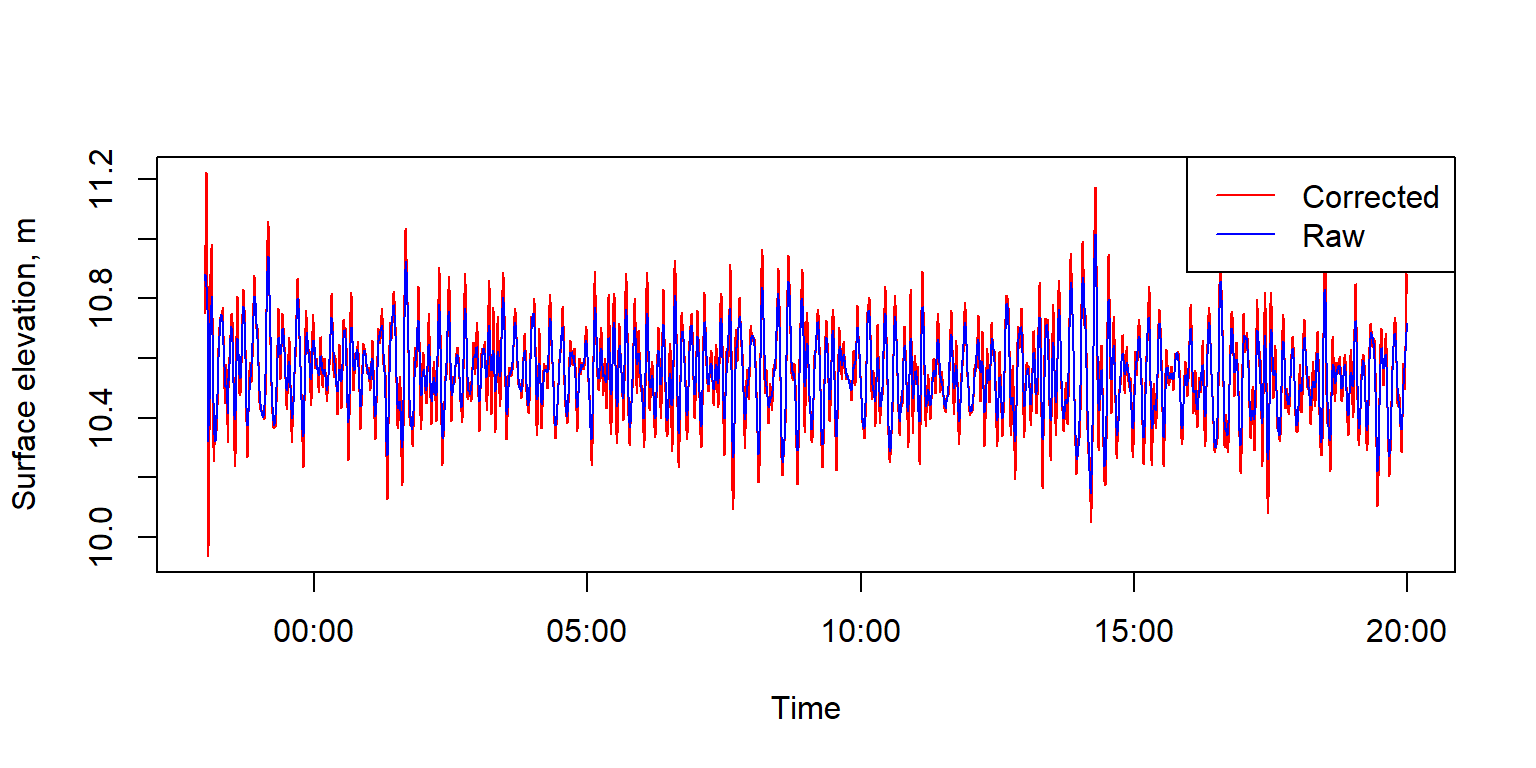
Comparison of the raw surface elevation (blue) and pressure-attenuation-corrected surface elevation (red). Pressure signal attenuation causes the true surface elevation fluctuation to be underestimated, and the correction attempts to undo that.
Below we’ll plot the short time series of sea surface elevations derived from our input csv files.
cols = '#E41A1C'  # red color
ylabloc = 3.2  # line location for y-axis labels
mybg = 'grey80' # color for plot backgrounds
op <- par(mar = c(4,6,1,1))
######################################
# Plot surface elevation record
plot(x = dat$DateTime,
        y = dat$swDepthCorrected.m,
        type = 'n', las = 1, ylab = '', xaxt='n',
        xlab = 'Time', col = cols)
rect(par()$usr[1],par()$usr[3],par()$usr[2],par()$usr[4],col=mybg)
grid(col ='white')
box()
lines(dat$DateTime,
        dat$swDepthCorrected.m, col = cols)
mtext(side = 2, line = ylabloc+0.7, text = 'Surface elevation, m')
axis(side=1,at = pretty(dat$DateTime),
     labels = format(pretty(dat$DateTime),format='%H:%M') )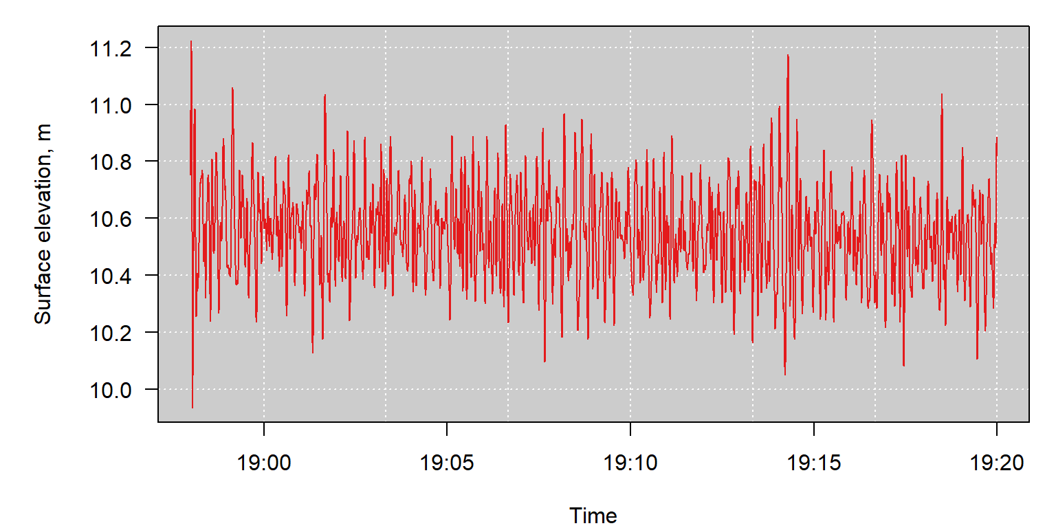
Time series of surface elevations.
par(op)At this point, the de-attenuated sea surface elevation data in the dat$swDepthCorrected.m column can be used to calculate various wave statistics.
Calculating wave statistics
Wave statistics are generally calculated for discrete chunks of time, often in the range of 15 to 30 minutes. If the original data were collected in non-contiguous chunks of time (such as a 15 minute sampling burst followed by 45 minutes of no data collection) then the time series in dat will already have natural boundaries for each burst to be analyzed due to gaps in the DateTime column values. If instead the data were collected continuously, as the OWHL is capable of doing, it would be necessary to create our own boundaries for each chunk of time to be analyzed. Our example data set in this vignette is short, so we will analyze the data in 5 minute chunks just for demonstration purposes.
The processBursts function takes several arguments. You need to provide a vector of sea surface elevations (in meters), a vector of POSIXct time stamps, the length of each burst you want to analyze (in minutes), the sampling rate of the sensor (default 4Hz for a OWHL), the method of analysis you want to use to generate the wave statistics (sp for spectral analysis, zc for zero-crossing wave-by-wave analysis), and the time zone of your input data.
# Go through each time chunk and calculate the wave
# height and period of the de-trended data (removing tide signal).

wavesSP = owhlR::processBursts(Ht = dat$swDepthCorrected.m,
                          times = dat$DateTime,
                          burstLength = 5,
                          Fs = 4,
                          method = 'sp',
                          tzone = 'UTC')
The results for the spectral analysis of wave data are shown below. The output includes:
h- Average water depth. Same units as input surface elevations (typically meters).Hm0- Significant wave height based on spectral moment 0. Same units as input surface heights (typically meters). This is approximately equal to the average height of the highest 1/3 of the waves.Tp- Peak period, calculated as the frequency with maximum power in the power spectrum. Units of seconds.m0- Estimated variance of time series (moment 0).T_0_1Average period calculated as \(\frac{m0}{m1}\), units seconds. Follows National Data Buoy Center’s method for average period (APD).T_0_2Average period calculated as \((\frac{m0}{m2})^{0.5}\), units seconds. Follows Scripps Institution of Oceanography’s method for calculating average period (APD) for their buoys.EPS2Spectral width parameter.EPS4Spectral width parameter.DateTimeThe date and time at the end of the burst.
wavesSP
#>          h       Hm0        Tp         m0    T_0_1    T_0_2      EPS2      EPS4
#> 1 10.57407 0.6408342 13.333333 0.02566678 8.737863 7.883985 0.4778501 0.7194574
#> 2 10.56416 0.5840060  7.058824 0.02131644 7.612516 7.085979 0.3926009 0.6060304
#> 3 10.54523 0.6002701 15.000000 0.02252026 8.792446 8.008976 0.4530091 0.6932817
#> 4 10.52990 0.7241655 13.333333 0.03277598 9.172730 8.399655 0.4387981 0.6862758
#>              DateTime
#> 1 2016-08-19 19:03:00
#> 2 2016-08-19 19:08:00
#> 3 2016-08-19 19:13:00
#> 4 2016-08-19 19:18:00
Wave climate estimates based on spectral analysis methods are probably the more commonly used method, but the wave-by-wave analysis using the zero-crossing method is provided for interested users.
# Go through each time chunk and calculate the wave
# height and period of the de-trended data (removing tide signal).

wavesZC = owhlR::processBursts(Ht = dat$swDepthCorrected.m,
                          times = dat$DateTime,
                          burstLength = 5,
                          Fs = 4,
                          method = 'zc',
                          tzone = 'UTC')
The output statistics from the zero crossing algorithm are:
Hsig- Mean height of the highest 1/3 of waves in the data set. Units = same as input surface elevations, usually meters.Hmean- Overall mean wave height, for all waves (bigger than threshold). Units = same as input surface elevations.H10- Mean height of the upper 10% of all waves. Units = same as input surface elevations.Hmax- Maximum wave height in the input data. Units = same as input surface elevations.Tmean- Mean period of all waves (bigger than threshold). Units of seconds.Tsig- Mean period ofHsig(highest 1/3 of waves). Units of seconds.DateTimeThe date and time at the end of the burst.
wavesZC
#>        Hsig     Hmean       H10      Hmax    Tmean      Tsig
#> 1 0.6486270 0.3998090 0.8180052 1.0485463 8.256944 10.229167
#> 2 0.5429659 0.3715567 0.6600402 0.7112625 7.187500  9.346154
#> 3 0.5750143 0.3652102 0.7228595 0.7837941 7.717105 10.000000
#> 4 0.6684549 0.4227043 0.8560766 1.1252348 8.104167 10.291667
#>              DateTime
#> 1 2016-08-19 19:03:00
#> 2 2016-08-19 19:08:00
#> 3 2016-08-19 19:13:00
#> 4 2016-08-19 19:18:00
Next we can plot the estimated significant wave heights from the two different analysis methods (spectral and zero-crossing) for each of the analyzed bursts.
ylims = range(c(wavesSP$Hm0,wavesZC$Hsig))
op<-par(mar=c(5,6,1,1))
plot(x = wavesSP$DateTime,y = wavesSP$Hm0, type = 'n',
     ylab = 'Significant wave\n height, m',
     xlab = 'Time',
     xaxt='n', las = 1, ylim = ylims)
rect(par()$usr[1],par()$usr[3],par()$usr[2],par()$usr[4],col=mybg)
grid(col ='white')
box()
lines(x = wavesSP$DateTime, y = wavesSP$Hm0, type = 'b')
axis(side=1,at = pretty(dat$DateTime),
     labels = format(pretty(dat$DateTime),format='%H:%M') )

lines(x = wavesZC$DateTime, y = wavesZC$Hsig, type = 'b',
      col = 'red')
legend('topleft',legend=c('Hm0, spectral method','Hsig, zero-cross'),
       col = c('black','red'), lty = c(1,1),
       pch = c(1,1))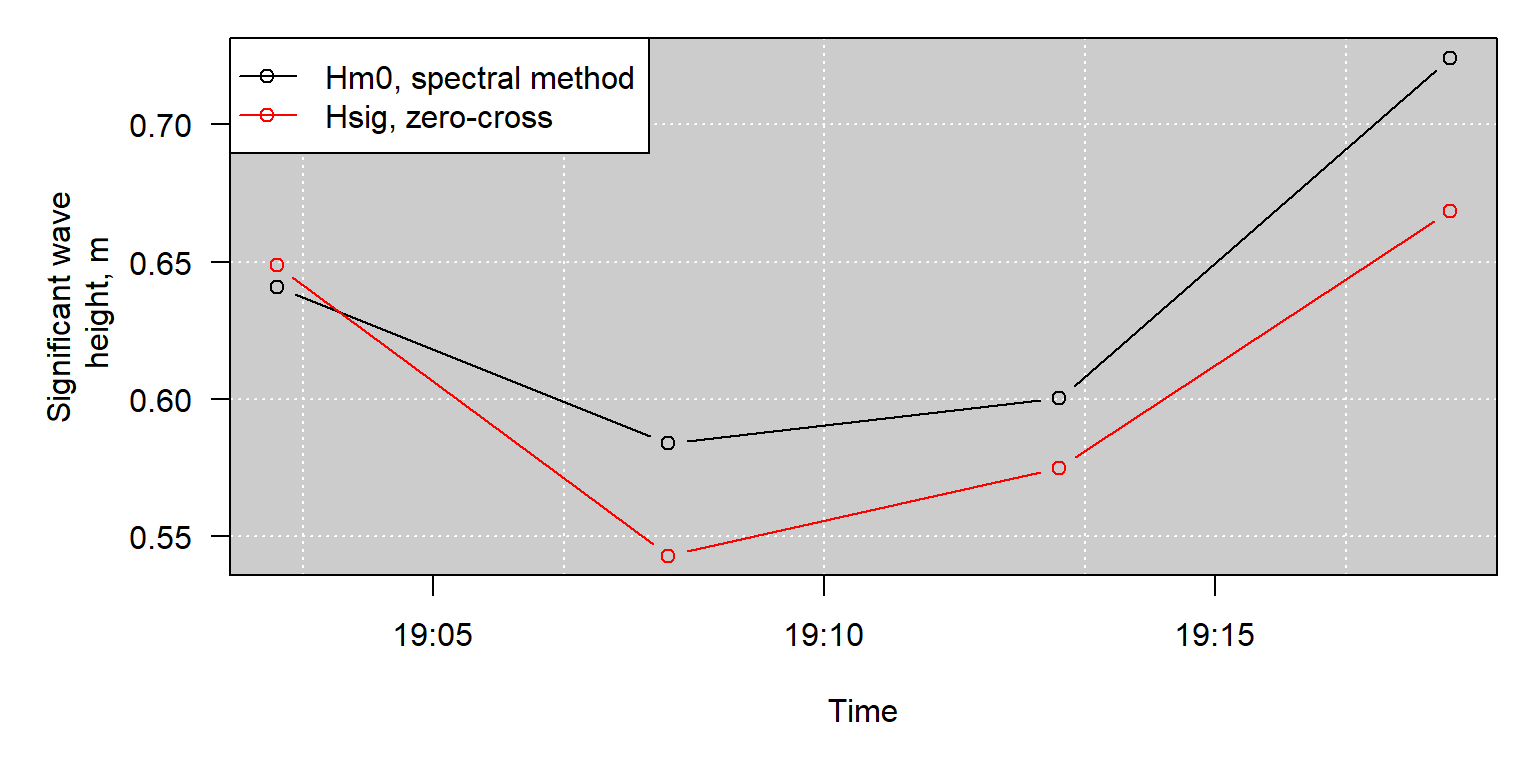
Estimates of signficant wave height from each analyzed burst of samples, using either the spectral analysis method or zero-crossing method.
par(op)ylims = c(3,25)
op<-par(mar=c(5,6,1,1))
plot(x = wavesSP$DateTime,y = wavesSP$Hm0, type = 'n',
ylab = 'Period, seconds',
xlab = 'Time',
xaxt='n', las = 1, ylim = ylims)
rect(par()$usr[1],par()$usr[3],par()$usr[2],par()$usr[4],col=mybg)
grid(col ='white')
box()
lines(x = wavesSP$DateTime, y = wavesSP$Tp, type = 'b')
axis(side=1,at = pretty(dat$DateTime),
labels = format(pretty(dat$DateTime),format='%H:%M') )
lines(x = wavesZC$DateTime, y = wavesZC$Tsig, type = 'b',
col = 'red')
legend('topleft',legend=c('Peak period, spectral method',
'Period of upper 1/3 of waves, zero-cross'),
col = c('black','red'), lty = c(1,1),
pch = c(1,1))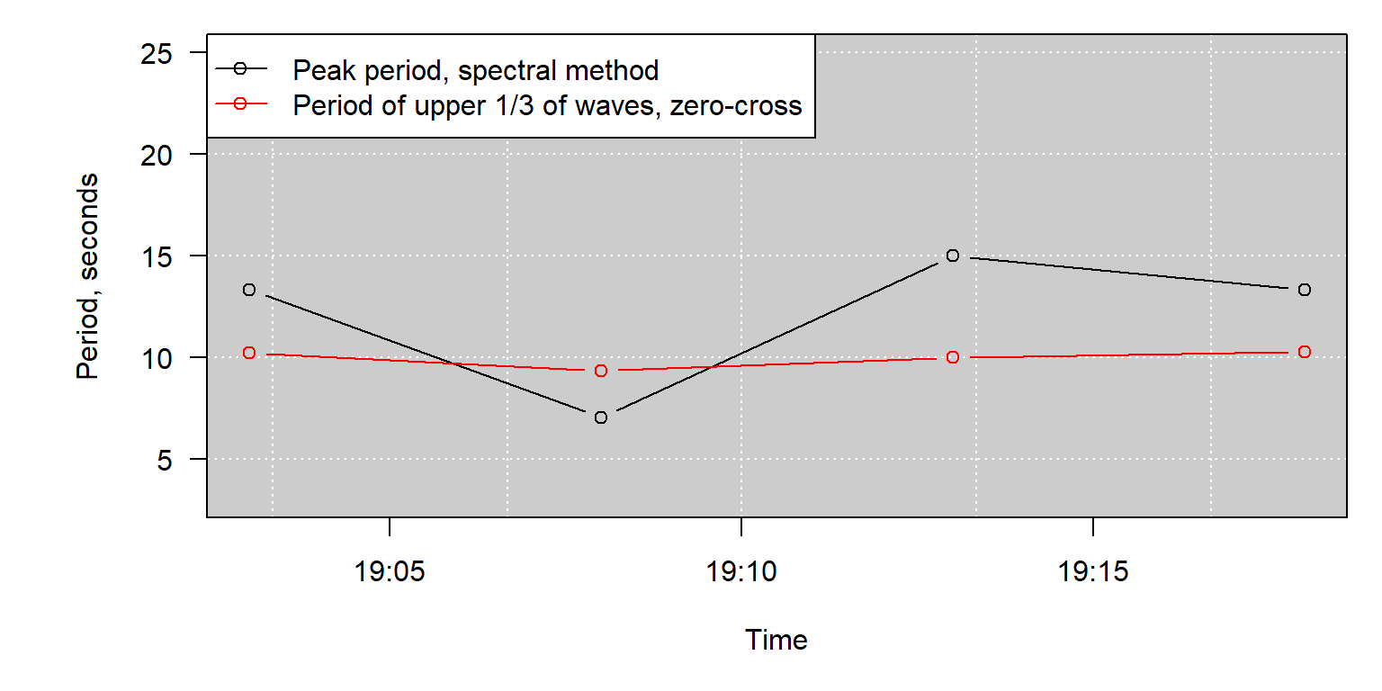
Estimates of wave period from each analyzed burst of samples, using either the spectral analysis method or zero-crossing method.
par(op)